About Learning I
“The answers you get depend upon the questions you ask.” - Thomas Kuhn.
Big Picture
Learning in Machine Learning is learning via computational methods using experience (data) to improve performance or to make accurate predictions.1
This learning is to automatically (minimal human intervention) discover regularities/patterns in data (through the use of computer algorithms) and with the use of these regularities to take actions (e.g. classifying the data into different categories)
Statistical Learning
Statistical learning refers to a vast set of tools for understanding data. These tools can be classified as supervised or unsupervised. Broadly speaking, supervised statistical learning involves building a statistical model for predicting, or estimating, an output based on one or more inputs. With unsupervised statistical learning, there are inputs but no supervising output; nevertheless we can learn relationships and structure from such data.2
Another way of understanding statistical learning is, it’s about studying the concept of inference (process of drawing conclusions from data) in both supervised and unsupervised machine learning. Inference covers the entire spectrum of machine learning, from gaining knowledge, making predictions or decisions and constructing models from a set of labeled or unlabeled data.
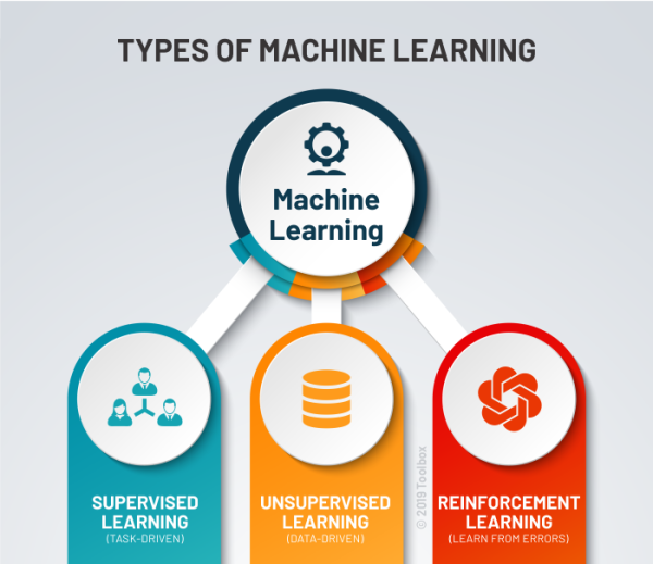
Supervised Learning: learning approach that’s defined by its use of labeled datasets. These datasets are designed to train or “supervise” algorithms into certain task (e.g. classifying data or predicting outcomes accurately)
Unsupervised Learning: learning strategy that’s looking for hidden or underlying patterns in datasets.
Reinforcement Learning: learning strategy which does not require labeled data or a training set. It relies on the ability to monitor the response to the actions of the learning agent. In general, a reinforcement learning agent is able to perceive and interpret its environment, take actions and learn through trial and error.
At the end we will measure success of this learning by some statistical model performance. This will tell whether our “trained” model is generalize(model’s ability to adapt properly to new, previously unseen data) well or not,
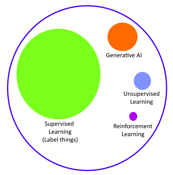
Figure 2 shows current AI opportunities. Andrew Ng highlight the opportunities in:
- AI for productivity : usage of Large Language Model (LLM) for office work
- AI for new products and services : to utilised AI to build previously unimaginable services and products.
We shall focus on Supervised Learning
The “problem setting” of statistical learning.
The basic setting of statistical learning is: given a problem statement, we want to find prediction model which estimate has best fit in providing solutions to the problem, using data at hand (in sample data) which has the Lowest Variance and Lowest Bias when applied to the data at hand as well as to the data not in hand (unseen data).
Vectors and Matrices
Vectors and matrices are fundamental mathematical structures that serve as the building blocks for representing and manipulating data in machine learning. They provide a concise and efficient way to organize, transform, and analyze complex datasets, enabling machine learning algorithms to make sense of raw information and extract meaningful patterns.
scalar: just a number, like 7, 42, \(\pi\). To a computer, a scalar is a simple numeric variable
vector: 1D array of numbers. Mathematically, a vector has an orientation, either horizontal or vertical. If horizontal, it’s a row vector. For example:
\[\textbf x = \begin{bmatrix} x_0 & x_1 & x_3 \end{bmatrix}\] Mathematically, vectors are usually assumed to be column vectors:
\[\textbf y = \begin{pmatrix} y_0 \\ y_1 \\ y_2 \\ y_3 \end{pmatrix}\] Either notation is acceptable. As we recall from SPM, vector usually have component (x,y and z) to represent a point in 3D space. However, in deep learning, and machine learning in general, vector are used to represent features, qualities of some sample that the model will use to attempt to arrive at a useful output, like a class label, or a regression value.
- matrices: 2D array of numbers:
\[\textbf A = \begin{bmatrix} a_{00} & a_{01} & a_{02} \\ a_{10} & a_{11} & a_{12} \end{bmatrix}\]
Example
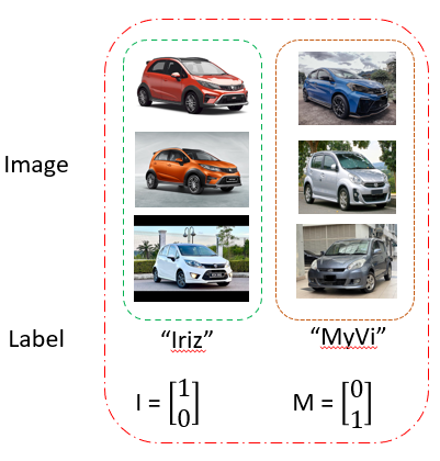
We will use the problem of car image classification as a running example to illustrate some basic definitions and to describe the use and evaluation of machine learning algorithms in practice. car image classification is the problem of learning to automatically classify 2 type of car image messages as either Perodua MyVi or Proton Iriz.
| Label | Description |
|---|---|
| 0 | MyVi |
| 1 | Iriz |
Examples: Items or instances of data used for learning or evaluation. In our problem, these examples correspond to the collection of car images we will use for learning and testing.
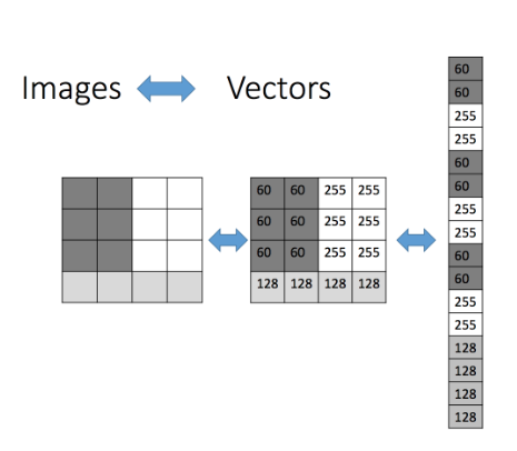
Features: The set of attributes, often represented as a vector, associated to an example. In the case of image classification, pixels are the raw building blocks of an image. Every image consists of a set of pixels. There is no finer granularity than the pixel. A pixel is considered the “color” or the “intensity” of light that appears in a given place in our image. Various location of this color will give texture, and shape.
Labels: Values or categories assigned to examples. In classification problems, examples are assigned specific categories, for instance, the Perodua MyVi and Proton Iriz categories in our binary classification problem.
Training sample: Examples used to train a learning algorithm. In our problem, the training sample consists of a set of car image examples along with their associated labels.
Validation sample: Examples used to tune the parameters of a learning algorithm when working with labeled data. Learning algorithms typically have one or more free parameters, and the validation sample is used to select appropriate values for these model parameters.
Test sample: Examples used to evaluate the performance of a learning algorithm. The test sample is separate from the training and validation data and is not made available (unseen data) in the learning stage.
Loss function: A function that measures the difference, or loss, between a predicted label and a true label. Also termed as objective function.
\(h\), (hypothesis): an instance or specific candidate model that maps inputs to outputs and can be evaluated and used to make predictions. A hypothesis is like a smart(well-informed) guess.
\(H\), Hypothesis set: set of conditions of specific candidate model that determines the classification into a group (a function approximation for the target function). It is a statement about the input data and its relation to the class. These “function” is used to associate/estimate or predict the target value, based on the input dataset, algorithm parameters (and hyper-parameters). Mathematically, it is a set of functions mapping features (feature vectors) to the set of labels Y. In our example, these may be a set of functions mapping car image features to Y = {MyVi, Iriz}.
model: A model can be viewed as a probabilistic model or as a non-probabilistic model(function). Every model has its own set of parameters(the weights and bias).
Learning is a search through the space of possible hypotheses for one that will perform well, even on new examples beyond the training set.3
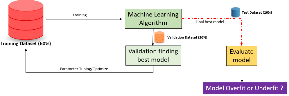
In Figure 4, we show generic statistical learning process.To ensure that our statistical model is going to perform well on new data, we need to consider the following:
- Using “user” prior knowledge, map relevant features of the collection of image into label/category
- Partition the data into a training sample, a validation sample, and a test sample.
- During training, example are drawn independently at random
- Our Machine learning algorithm now analyze the examples and produce a classifier,\(f\)
- given new example from validation, classifier,\(f\) predict \(\hat{y}=f(x)\)
- Measure loss between real truth, \(y\) and predicted,\(\hat{y}\)
- If loss high, repeat (3)-(6) until loss is minimize.
What happen at step (4) - step (6)
To have rough idea what’s going on at step (4), consider Figure 5 where our data is label as vector(step (1)).
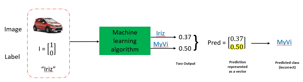
Thus in Figure 6, during 1 individual training loop. Prediction vector is later will be compare with data label using loss function and error is compute.
Interpret step (6)
Bias : amount that a model’s prediction differs from the target value, compared to the training data.
Low Bias: fewer strong assumptions or constraints placed during model training. In this case, the model will closely match the training dataset. Model has ability to capture the true underlying patterns or relationships present in the data
High Bias : model simplifies the underlying patterns too much (strong assumptions or constraints placed during model training). In this case, the model will not match the training dataset closely. Usually called under-fitting
Variance: the variability of the model that how much it is sensitive to another subset of the training dataset. i.e. how much it can adjust on the new subset of the training dataset.
Low Variance : not overly influenced by the noise or fluctuations in the training data. It tends to be more stable, providing consistent predictions even when trained on different subsets of the data.
High Variance : overly sensitive to the noise or fluctuations in the training data. It tries to fit the training data so closely that it captures not only the true underlying patterns but also the random noise in the data. Usually called over-fitting
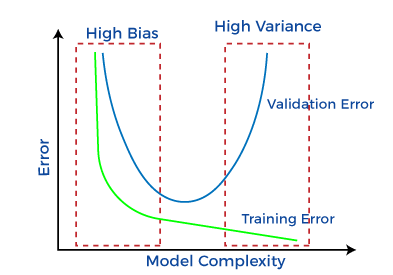
High Bias and Low Variance: Consistent but inaccurate due to oversimplification. \(\Longrightarrow\) poor performance
High Variance and Low Bias: Accurate but inconsistent, capturing noise and over-fitting to the training data. \(\Longrightarrow\) poor performance
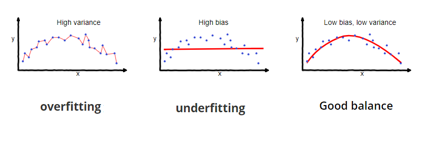
Overfitting is when your model is basically memorising the data without really understanding/interpolating a general function that would apply to any external data. In other words it creates a function that is tailored specifically to the training dataset thus it would perform near perfectly with the training data, but it would perform quite badly with any data that it hasn’t seen before. (models the training data too well but fails to generalize to new data)
Underfitting is simply when you do not have enough data for the model to create/interpolate a general function that describes the process. This leads to the model performing badly for most input data. (model that fails to capture the underlying pattern in the training data)
- What do we want? \(\Longrightarrow\) To make predictions on unseen data \(\Longrightarrow\) We want a model that generalizes well \(\Longrightarrow\) generalizes to unseen data
- How we will do this? \(\Longrightarrow\) controlling the complexity of the model (learning parameter)
- How do we know if our model generalizes? \(\Longrightarrow\) evaluating on test data.
Learning is NOT memorization! The ability to produce correct outputs on previously unseen inputs is called generalization